Using
a Spreadsheet to Analyse Statistics
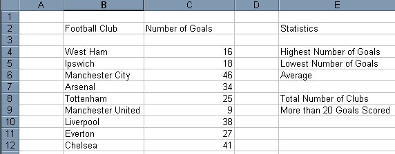
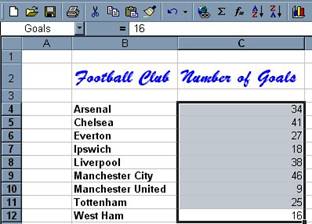
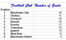
In this tutorial, you will enter data about the number
of goals scored by various football teams and you will carry out statistical
analysis on the data.
1. Entering the Data
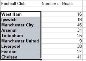
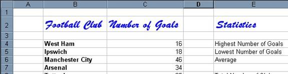
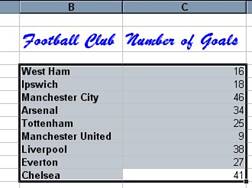
1. Enter the data as shown below.
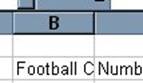
2. Some of the columns will not be wide enough. To remedy this, re-size the columns or double-click on the intersection between the column headings. See below:

Double-click
here
3. Highlight the names of the teams and click the Bold button on the Excel toolbar.
2. Using the Format
Painter
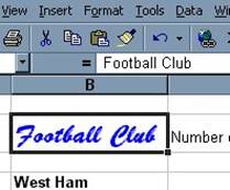
1. Make the heading “Football Club” blue, bold and change the font to Brush Script (or another font of your choice). Make the font slightly bigger.
2. Make sure cell B2 is still selected and double-click the Format Painter button

Format Painter Button
3. Then click once on cells C2 and E2, which also contain column headings. Adjust the width of the columns again, as necessary.
4. Deselect the Format Painter button.
The Format Painter is also available in other Microsoft Office applications, such as Word, Publisher and Access.
3. Sorting the Data
You notice that the teams are not listed in alphabetical order and you decide that you want to put this right.
1. You must first select columns B and C
It is very important that you do this. If you just sort the list of team names, the teams will be rearranged but the goals scored won’t. That would make your data incorrect.
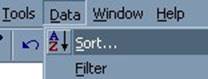
2. From the Data menu, select Sort.
3. Sort by Column B (the teams list) and do an Ascending sort (A-Z)
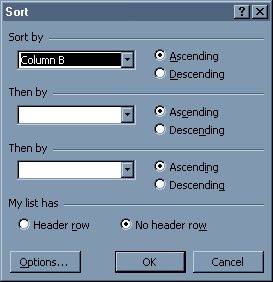
The teams should now be listed in alphabetical order and the number of goals scored for each team should be correct.
4. The MAX and MIN
Functions
1. Select the cells that contain the number of goals scored and enter “Goals” in the Name Box and then hit the Enter key.
Name Box
![]()
From now on, you can enter Goals instead of the cell range (C4:C12)
2. Click in Cell F4
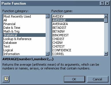
3. Start the Function Wizard by clicking the button on the toolbar:
![]()
4. In the Function Category select Statistical and for Function Name select Max.
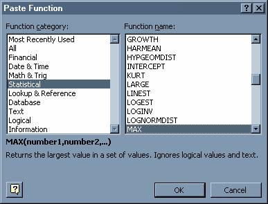
5. Click OK
6. Enter Goals
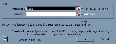
7. The highest number of goals scored (46) should now be displayed in cell F4
In cell F5 you want to have the lowest number of goals displayed. You can achieve this by using the MIN function:
8. Click in cell F5
9. Start the Function
Wizard
![]()
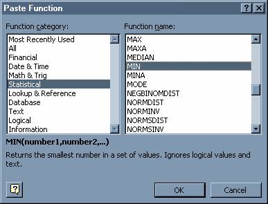
10. Select the MIN
function from the Statistical category and click OK
11. Enter the range Goals
12. Click OK and the lowest number of goals scored (9) is displayed in cell F5
5. The Average Function
In cell F6 you want Excel to display the average number of goals scored. You will do this by using the Average function.
1. Click in cell F6
2. Start the Function
Wizard
![]()
3. Select the Average function from the Statistical category
4. Click OK
5. Enter the range Goals
6. Click OK and the average number of goals scored should be displayed in F6
7. To stop Excel displaying the number of decimal places, make sure that F6 is still selected and click the Decrease Decimal
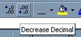
Remove all the decimal places and you should be left with the number 28 being displayed in F6
6. Calculating Functions
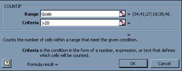
To calculate how many teams are included and how many teams have scored more than 20 goals, we will use the COUNTA and COUNTIF functions.
1. Entering the COUNTA function is just as easy as entering the MAX, MIN and AVERAGE functions. You can do this by starting the Function Wizard and selecting COUNTA from the Statistical category.
However, there is a quicker way to do it. Just type =COUNTA(Goals) into cell F8.
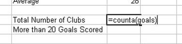
Hit the ENTER key on your keyboard and the number of teams is displayed.
2. The COUNTIF function is slightly more complicated, so we will use the Function Wizard this time. Start the Function Wizard and select COUNTIF from the Statistical category.
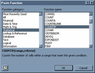
3. Enter Goals as the range and >20 as the criteria (Excel will count the number of teams who have scored more than 20 goals. Finally click OK.
7. Extension Activities
1. Every week, you are going to update the number of goals scored. Excel will then update the calculations automatically. After a few more games, the number of goals has changed. Change the number of goals scored by each team on your table, as follows:
Arsenal 40
Everton 35
Tottenham 29
West Ham 20
2. Add a function to display the number of teams who have scored more than 30 goals.
3. Change the COUNTIF function in cell F9 so that it displays the number of teams to have scored “20 or more” goals.
Hint: you need to change the Criteria used in the function. The following list of acceptable criteria will be useful:
More than 20 >20
More or equal to 20 >=20
Less than 20 <20
Less than or equal to 20 <=20
4. Add a function to show the number of teams to have scored less than 20 goals.
5. Add an extra team to your list
Name of team:
Goals Scored: 26
Sort the list so that the teams are listed in order of the number of goals scored. Remember you have to select both data columns.
Has the number of teams in cell F9 increased to 10? Why not? This is going to take some thought on your part!
Hint: Select Name/Define from the Insert menu
6. See if you can get Excel to automatically display a “Best Team” and a “Worst Team”, as follows:
![]()
Hint: the solution to this one is extremely simple!
7. Use the Rank Function to show the position of each team in the table.
Hint to get you
started: the formula in cell A4 is =RANK(C4,goals,0)
8. Create some calculation formulas to show
the number of goals scored by
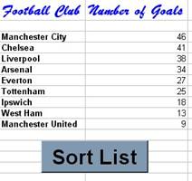
9. You can automatically sort the list of teams by creating a macro button, as follows:
· You need to view the Forms Toolbar (View/Toolbars/Forms)
· Add a button and label it “Sort List”
· From the Tools menu, select Macro/Record New Macro
· Give the Macro a name and start recording
· Sort the list and then stop the recording
· Click the Right Mouse Button on the Sort Button
· Assign the macro you created to the button
· Finally, test your button and make sure it works
10. How else could this spreadsheet be developed? Use your imagination!